Uniform logarithmic Sobolev inequalities for the 2D Coulomb gas at the diffusive temperature scale, Part I
Download the archival PDF version of this post.
This is the first of two posts on uniform logarithmic Sobolev inequalities for the planar Coulomb gas at the diffusive temperature scale. Here, I explain our first, perturbative proof, both because it already gives a complete uniform result at small inverse temperature and because the places where it stops isolate the analytic problem that must be solved to reach every fixed inverse temperature.
1 The problem and a first uniform theorem
For \(N\ge2\) and a fixed inverse temperature \(\beta>0\), consider the canonical Gibbs ensemble \(\mathbb{P}_{N,\beta}\) on the full labeled configuration space \(\mathbb C^N\simeq(\mathbb R^2)^N\). Here, “canonical” means that the particle number is fixed. We write
\[ \mathsf g(z):=-\log|z| \tag{1.1} \]
for the planar logarithmic Coulomb kernel, and define
\[ \,\mathrm d\mathbb{P}_{N,\beta}(Z) =\frac1{Z_{N,\beta}} \exp\!\left(-\frac\beta2\sum_{i=1}^N|z_i|^2\right) \prod_{1\le i<j\le N}|z_i-z_j|^{\beta/N}\,\,\mathrm dZ. \tag{1.2} \]
Equivalently,
\[ \mathcal H_N(Z) =\frac12\sum_{i=1}^N|z_i|^2 +\frac1N\sum_{1\le i<j\le N}\mathsf g(z_i-z_j), \qquad \mathbb{P}_{N,\beta}\propto e^{-\beta\mathcal H_N}\,\mathrm dZ. \tag{1.3} \]
Since \(\mathsf g(z)\to+\infty\) as \(z\to0\), the interaction is repulsive and the density vanishes at collisions.
The factor \(1/N\) in (1.3) places the system at the diffusive temperature scale. The reversible overdamped Langevin dynamics is formally
\[ \,\mathrm dZ_i(t) =-\left(Z_i(t)-\frac1N\sum_{j\ne i} \frac{Z_i(t)-Z_j(t)}{|Z_i(t)-Z_j(t)|^2}\right)\,\mathrm dt +\sqrt{\frac2\beta}\,\,\mathrm dB_i(t), \tag{1.4} \]
and the noise amplitude remains of order one as \(N\to\infty\). This differs from the usual random-matrix scaling (see, e.g., [Ser24]), where the Gibbs exponent is of order \(N^2\) and the effective noise vanishes with the particle number.
For a probability measure \(\mathbb P\), set
\[ \mathop{\mathrm{Ent}}_{\mathbb P}(f^2) :=\int f^2\log\!\left(\frac{f^2}{\int f^2\,\mathrm d\mathbb P}\right)\,\mathrm d\mathbb P. \tag{1.5} \]
Our convention for the logarithmic Sobolev constant is
\[ \mathop{\mathrm{Ent}}_{\mathbb{P}_{N,\beta}}(f^2) \le \frac2{\rho_{N,\beta}} \int_{\mathbb C^N}|\nabla f|^2\,\mathrm d\mathbb{P}_{N,\beta}. \tag{1.6} \]
The domain in (1.6) requires some care because the density vanishes at collisions. Let
\[ \mathcal C_N:=\{Z\in\mathbb C^N:z_i=z_j\text{ for some }i\ne j\}, \qquad \Omega_N:=\mathbb C^N\setminus\mathcal C_N, \tag{1.7} \]
and, initially for \(f\in C_c^\infty(\Omega_N)\), set
\[ \mathcal E_{N,\beta}(f) :=\int_{\Omega_N}|\nabla f|^2\,\mathrm d\mathbb{P}_{N,\beta}, \qquad \|f\|_{N,\beta}^2 :=\int_{\mathbb C^N}|f|^2\,\mathrm d\mathbb P_{N,\beta}+\mathcal E_{N,\beta}(f). \tag{1.8} \]
We denote the closed form domain by
\[ \mathsf D_{N,\beta} :=\overline{C_c^\infty(\Omega_N)}^{\,\|\cdot\|_{N,\beta}} =\overline{C_c^\infty(\mathbb C^N)}^{\,\|\cdot\|_{N,\beta}}. \tag{1.9} \]
The second equality follows from the zero-capacity argument in Section 2. Thus, \(\mathsf D_{N,\beta}\) is the full closed weighted Sobolev domain, with no boundary condition imposed at collisions.
The question is whether, for each fixed \(\beta>0\), one can find
\[ \rho_*(\beta)>0 \quad\text{such that}\quad \rho_{N,\beta}\ge\rho_*(\beta) \qquad\text{for every }N\ge2. \tag{1.10} \]
We impose no symmetry or other structural assumption on the observable \(f\).
To identify where particle-number dependence can enter, we first separate the center of mass. In the present quadratic setting, this separation is exact. Set
\[ c_N:=\frac1{\sqrt N}\sum_{i=1}^Nz_i, \qquad Z^{\mathrm{rel}} :=Z-\frac{c_N}{\sqrt N}(1,\ldots,1). \tag{1.11} \]
Then,
\[ |Z|^2=|c_N|^2+|Z^{\mathrm{rel}}|^2, \qquad \prod_{i<j}(z_i-z_j) =\prod_{i<j}(z_i^{\mathrm{rel}}-z_j^{\mathrm{rel}}). \tag{1.12} \]
Thus, \(\mathbb P_{N,\beta}\) factors into a two-dimensional Gaussian proportional to \(e^{-\beta|c_N|^2/2}\,\mathrm dc_N\) and a Gibbs measure on the relative hyperplane \(\{\sum_i z_i=0\}\). The Gaussian factor has Poincaré cost \(1/\beta\) and logarithmic Sobolev rate \(\beta\); all of the nontrivial work lies in the relative coordinates.
For each fixed \(N\), a qualitative logarithmic Sobolev inequality follows from the existing Lyapunov theory, as we explain in Section 2. The difficulty is quantitative: the fixed-dimensional argument gives no reason for its constant to remain positive while the ambient dimension and the number of collision strata grow with \(N\).
Set
\[ \beta_{\mathrm B} :=\frac{8}{\pi^2+8} =0.4476875828047043\ldots. \tag{1.13} \]
The subscript records the integrated Bochner estimate from which this particular number arises.
The main result of this post is the following uniform logarithmic Sobolev inequality at small inverse temperature.
Theorem 1 Theorem 1.1 (Perturbative uniform logarithmic Sobolev inequality). *For every \(0<\beta\le\beta_{\mathrm B}\), there exists \(\rho_\beta>0\), depending on \(\beta\) but not on \(N\), such that
\[ \mathop{\mathrm{Ent}}_{\mathbb{P}_{N,\beta}}(f^2) \le\frac2{\rho_\beta} \int_{\mathbb C^N}|\nabla f|^2\,\mathrm d\mathbb{P}_{N,\beta} \tag{1.14} \]
for every \(N\ge2\) and every \(f\in\mathsf D_{N,\beta}\).*
A later refinement of the same perturbative strategy extends Theorem 1.1 to every \(0<\beta<1\). We will explain that improvement in Section 6. The first proof remains worth presenting because its numerical threshold is determined by a single inequality needed to close the estimate, while the rest of the argument already has the form used later.
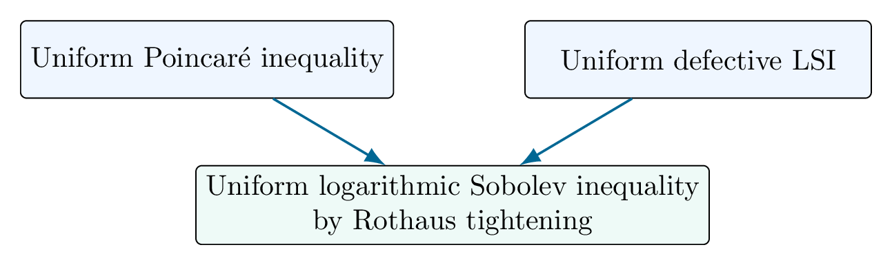
The strategy of the proof is classical: one proves a uniform Poincaré inequality and, independently, a defective logarithmic Sobolev inequality, and then removes the defect by Rothaus’s centering argument [Rot85]. Uniformity comes from the two input estimates, not from the tightening step itself.
2 Relation with existing work
The relevant literature is best understood in terms of proof mechanisms rather than as a linear progression of increasingly weak hypotheses. The classical dimension-free theory begins with the Gaussian logarithmic Sobolev inequality, tensorization, hypercontractivity, the Bakry–Émery curvature criterion, and bounded perturbation; see Gross [Gro75], Holley–Stroock [HS87], and Bakry–Gentil–Ledoux [BGL14]. For broader treatments of functional inequalities and concentration, see also [ABC+00, Led01]. Weakly coupled and multiscale Gibbs systems are instead treated by assembling one-site or block inequalities with a quantitative interaction estimate, as in the Dobrushin–Zegarlinski theory, the Otto–Reznikoff criterion, and two-scale decompositions [GZ03, OR07, GOVW09].
For regular mean-field particle systems, recent proofs use flat convexity, conditional coercivity, reverse-heat-flow transport, uniform spectral gaps, or a free-energy decomposition; representative works include [GLWZ22, Wan24, CNZ24, Mon24, BBD25]. These theories typically require global control of the interaction field, an \(L^\infty\) bound for its Hessian, or a worst-case influence matrix. The logarithmic kernel presents two distinct obstructions: its gradient and Hessian diverge at collisions, while at every nonzero separation its Hessian has one positive and one negative eigenvalue. Thus, the interaction is neither convex nor concave even off the collision set.
Singular one-dimensional systems admit a different mechanism. Chafaï–Lehec [CL20] and my work with Serfaty [RS25] exploit ordering, convexity on a Weyl chamber, and one-dimensional transport or rigidity. In the plane, particles can pass around one another without crossing the collision set, so there is no analogous global chamber decomposition.
The closest dynamical antecedents are the planar Coulomb works of Bolley–Chafaï–Fontbona [BCF18] and Lu–Mattingly [LM20]. The former study the overdamped dynamics and prove fixed-\(N\) functional and ergodic estimates. The latter write down the overdamped system, identify the potential energy as its natural Lyapunov function, and develop the collision-sensitive force estimates in the kinetic setting. These results make the following qualitative statement essentially part of the existing Lyapunov folklore, even though the exact formulation does not seem to have been written down explicitly in the literature.
Proposition 2.1 (Fixed particle number LSI). For every fixed \(N\ge2\) and \(\beta>0\), the measure \(\mathbb{P}_{N,\beta}\) in (1.2) satisfies a logarithmic Sobolev inequality on \(\mathsf D_{N,\beta}\). The constant may depend arbitrarily badly on \((N,\beta)\).
We make no novelty claim for Proposition 2.1. Bolley–Chafaï–Fontbona explicitly point to the local-to-global Lyapunov route and the collision-domain difficulty [BCF18, Section 1.4.5]; the abstract mechanism is developed in [CG14, CGWW09, CG17]. Here is a sketch of the proof.
Finiteness and capacity at collisions. Here, capacity means the variational \(1\)-capacity associated with the weighted Dirichlet form and its form norm; see [FOT11, Section 2.1]. Fix \(i<j\), set \(\alpha:=\beta/N\), and choose a smooth function \(\chi\) equal to one on \([0,1]\) and zero on \([2,\infty)\). For \(u_{ij,\varepsilon}(Z):=\chi(|z_i-z_j|/\varepsilon)\), the cutoff equals one near the collision divisor and satisfies \(|\nabla u_{ij,\varepsilon}|^2\le C\varepsilon^{-2}\). Writing \(w=z_i-z_j\in\mathbb R^2\), the Gibbs density contributes the factor \(|w|^\alpha\), while polar coordinates contribute the Jacobian \(r\,\mathrm dr\,\mathrm d\theta\). The remaining variables have an \(\varepsilon\)-independent integrable majorant, owing to the Gaussian confinement. Therefore, \[\mathcal E_{N,\beta}(u_{ij,\varepsilon}) \le C\varepsilon^{-2}\int_\varepsilon^{2\varepsilon}r^{\alpha+1}\,\mathrm dr \le C\varepsilon^\alpha\longrightarrow0.\] Likewise, \[\int_{\mathbb C^N}|u_{ij,\varepsilon}|^2\,\mathrm d\mathbb P_{N,\beta} \le C\int_0^{2\varepsilon}r^{\alpha+1}\,\mathrm dr \le C\varepsilon^{\alpha+2}\longrightarrow0.\] Thus, every collision divisor has zero weighted capacity. Since the full collision set is a finite union of these divisors, it also has zero capacity. Equivalently, cutoffs vanishing near the full collision set converge to one in the form norm, which proves the second equality in (1.9).
Lyapunov coercivity. Let
\[ \mathcal L=\Delta-\beta\nabla \mathcal H_N\cdot\nabla. \tag{2.1} \]
On \(\Omega_N\), if \(W=e^{a\mathcal H_N}\) with \(0<a<\beta\), then
\[ \frac{\mathcal LW}{W} =a\Delta \mathcal H_N-a(\beta-a)|\nabla \mathcal H_N|^2. \tag{2.2} \]
Because \(-\log|z|\) is harmonic away from the origin,
\[ \Delta \mathcal H_N=2N \qquad\text{on }\Omega_N. \tag{2.3} \]
The singular Coulomb forces remain collectively large as a bounded configuration approaches the collision set, despite possible cancellations among individual pair forces. Together with quadratic confinement at infinity, this makes the energy gradient coercive outside a compact subset of the collision-free configuration space. The simpler identity
\[ Z\cdot\nabla \mathcal H_N(Z)=|Z|^2-\frac{N-1}{2} \tag{2.4} \]
shows the tail mechanism directly: for \(\Phi(Z)=|Z|^2/2\),
\[ \mathcal L\Phi =2N-\beta|Z|^2+\frac{\beta(N-1)}2. \tag{2.5} \]
This radial Lyapunov function does not control collisions by itself, which is why the singular force estimate is still needed.
From local to global. The region where the Lyapunov drift is not coercive is compactly contained in \(\Omega_N\). On a connected neighborhood of that compact set, the density is smooth and bounded above and below, so ordinary local Poincaré and Sobolev inequalities apply. The local-to-global argument yields a defective logarithmic Sobolev inequality and a fixed-\(N\) Poincaré inequality; Rothaus tightening then gives the stated LSI.
We emphasize that every constant in the preceding argument may depend on the ambient dimension \(2N\), the number of collision divisors, the compact set on which local coercivity is invoked, and the Lyapunov threshold. Thus, the uniform LSI we will show should not be viewed as an optimization of Proposition 2.1. Rather, it requires a new approach in which the particle-number dependence cancels explicitly.
3 Conditional weighted inequalities and labeled fluctuations
The logarithmic interaction has an important structural property: after conditioning on all but one particle, or all but one pair, the remaining density is a Gaussian multiplied by positive powers of distances to finitely many points or affine subspaces. The number of factors grows with \(N\), but, since \(\beta\) is held fixed as \(N\to\infty\), their exponents add to a quantity of order one. Up to this point, only the logarithmic form of the interaction has been used and not the fact that we are in a planar setting. The latter enters later through the circle estimate, complex analysis, and the two-dimensional weighted theory discussed in Section 6.
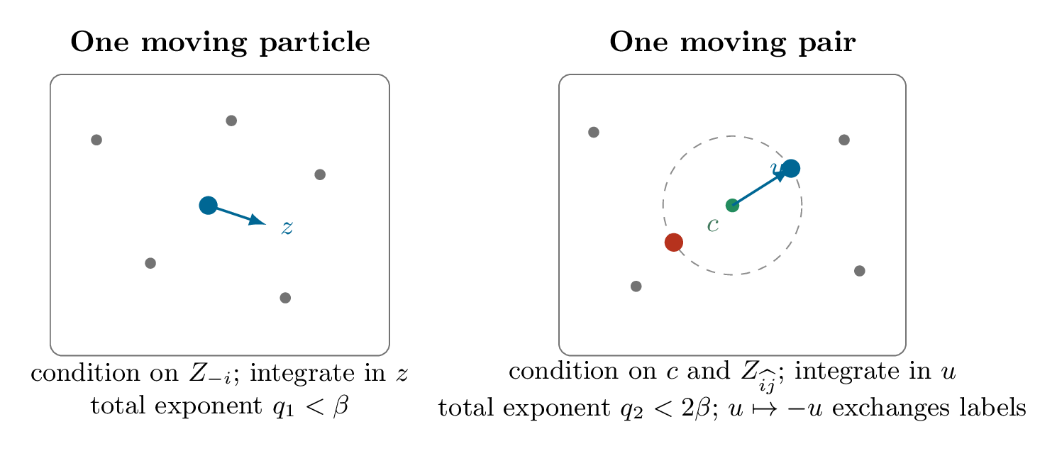
Condition first on \(Z_{-i}:=(z_j)_{j\ne i}\). The one-site conditional law is
\[ \,\mathrm d\mathbb{P}_i(z\mid Z_{-i}) \propto e^{-\beta|z|^2/2} \prod_{j\ne i}|z-z_j|^{\beta/N}\,\,\mathrm dz, \tag{3.1} \]
whose distance factors have total exponent
\[ q_1:=\sum_{j\ne i}\frac\beta N =\frac{\beta(N-1)}N<\beta. \tag{3.2} \]
Here and below, the total exponent means the sum of the powers appearing in a product of distance factors. In the sequel, we will refer to the \(\varepsilon\)-regularization of a factor \(|\xi|^\alpha\), meaning its replacement by \((|\xi|^2+\varepsilon^2)^{\alpha/2}\), with \(\varepsilon>0\).
3.1 A brief weighted-analysis interlude
To turn the preceding observation into a functional inequality, we use the Muckenhoupt classes. Let \(1<p<\infty\). A locally integrable weight \(w\) satisfying \(0<w<\infty\) a.e. on \(\mathbb R^d\) belongs to \(A_p(\mathbb R^d)\) if and only if
\[ [w]_{A_p} :=\sup_B \left(\frac1{|B|}\int_Bw\,\mathrm dx\right) \left(\frac1{|B|}\int_Bw^{-1/(p-1)}\,\mathrm dx\right)^{p-1} <\infty, \tag{3.3} \]
where the supremum is over Euclidean balls (equivalently, cubes). We also set
\[ A_\infty:=\bigcup_{1\le p<\infty}A_p. \tag{3.4} \]
Muckenhoupt introduced these classes in [Muc72]; see Grafakos [Gra14, Chapter 9] for a modern treatment.
The conditional weighted estimates used in Part I are based on the class \(A_2\); that is, we use \(p=2\). The model criterion
\[ |x|^\alpha\in A_p(\mathbb R^d) \quad\Longleftrightarrow\quad -d<\alpha<d(p-1) \tag{3.5} \]
shows in particular that
\[ |x|^q\in A_2(\mathbb R^2) \quad\Longleftrightarrow\quad -2<q<2. \tag{3.6} \]
At the upper endpoint, the reciprocal weight ceases to be locally integrable. The weighted Poincaré and Sobolev inequalities of Fabes–Kenig–Serapioni (3.4); see David–Semmes [DS90].
For the conditional measure (3.1), the ambient \(A_2\) estimate is combined with a radial reciprocal-weight bound, a Gaussian Hardy estimate, and a super-Poincaré globalization. The stricter radial threshold is \(q_1<1\), and this gives the following uniform statement.
Proposition 3.1 (Uniform one-site conditional LSI). *Let \(0<\beta<1\). There is \(\rho_1(\beta)>0\), independent of \(N\), the index \(i\), and the conditioned positions \(Z_{-i}\), such that
\[ \mathop{\mathrm{Ent}}_{\mathbb{P}_i(\cdot\mid Z_{-i})}(h^2) \le\frac2{\rho_1(\beta)} \int_{\mathbb C}|\nabla h|^2\,\mathrm d\mathbb{P}_i(\cdot\mid Z_{-i}) \tag{3.7} \]
for every \(h\) in the conditional Dirichlet-form domain.*
3.2 One moving pair
The first, perturbative proof also uses a two-particle conditional inequality. To formulate it, fix distinct indices \(i\) and \(j\) and condition on all remaining coordinates. Given
\[ Z_{\widehat{ij}}:=(z_k)_{k\notin\{i,j\}}, \tag{3.8} \]
the two-particle conditional law is
\[ \,\mathrm d\mathbb P_{ij}(z,w\mid Z_{\widehat{ij}}) \propto e^{-\beta(|z|^2+|w|^2)/2}|z-w|^{\beta/N} \prod_{k\ne i,j}|z-z_k|^{\beta/N}|w-z_k|^{\beta/N}\,\,\mathrm dz\,\,\mathrm dw. \tag{3.9} \]
As a weight on \(\mathbb R^4\simeq\mathbb C^2\), its distance factors vanish on affine subspaces of real codimension two. Their total exponent is
\[ q_2:=\frac\beta N\bigl(1+2(N-2)\bigr) =\frac{\beta(2N-3)}N<2\beta. \tag{3.10} \]
Proposition 3.2 (Uniform two-particle conditional LSI). *Let \(0<\beta<1/2\). There is \(\rho_2(\beta)>0\), independent of \(N\), the pair \((i,j)\), and \(Z_{\widehat{ij}}\), such that
\[ \mathop{\mathrm{Ent}}_{\mathbb P_{ij}(\cdot\mid Z_{\widehat{ij}})}(h^2) \le\frac2{\rho_2(\beta)} \int_{\mathbb C^2}\bigl(|\nabla_z h|^2+|\nabla_w h|^2\bigr) \,\mathrm d\mathbb P_{ij}(\cdot\mid Z_{\widehat{ij}}). \tag{3.11} \]
The same estimate holds after this \(\varepsilon\)-regularization, with the same constant uniformly in \(\varepsilon>0\).*
The fixed-dimensional Gaussian affine-subspace theorem applies when the total exponent is bounded strictly below one. Since \(q_2<2\beta\), this gives the uniform margin \(\beta<1/2\) used in the first proof.
A more economical reduction will be needed for the later improvement to \(\beta<1\). Introduce the orthogonal pair coordinates
\[ c_{ij}:=\frac{z_i+z_j}{\sqrt2}, \qquad u_{ij}:=\frac{z_i-z_j}{\sqrt2}. \tag{3.12} \]
Condition further on \(c_{ij}\) and \(Z_{\widehat{ij}}\), and write \(c=c_{ij}\) and \(u=u_{ij}\). If
\[ A_k:=\frac c{\sqrt2}-z_k, \qquad k\ne i,j, \tag{3.13} \]
then
\[ (z_i-z_k)(z_j-z_k)=A_k^2-\frac{u^2}{2}, \qquad z_i-z_j=\sqrt2\,u. \tag{3.14} \]
The conditional law of \(u\) is therefore proportional to
\[ e^{-\beta|u|^2/2} \left|u\prod_{k\ne i,j}\left(A_k^2-\frac{u^2}{2}\right)\right|^{\beta/N}\,\mathrm du. \tag{3.15} \]
Each quadratic factor has the two roots \(u=\pm\sqrt2\,A_k\). Thus, together with the root at zero, the conditional weight contains \(2N-3\) linear distance factors, each with exponent \(\beta/N\); their total exponent is \(q_2\).
Proposition 3.3 (Uniform relative-coordinate Poincaré inequality). *Let \(0<\beta<1\). There is \(C_{\mathrm{rel}}(\beta)<\infty\), independent of \(N\), the pair \((i,j)\), the conditioned center \(c_{ij}\), and \(Z_{\widehat{ij}}\), such that
\[ \mathop{\mathrm{Var}}_{\mathbb P_{ij}^{\mathrm{rel}}}(h) \le C_{\mathrm{rel}}(\beta) \int_{\mathbb C}|\nabla h|^2\,\mathrm d\mathbb P_{ij}^{\mathrm{rel}}. \tag{3.16} \]
The estimate is also uniform in \(\varepsilon>0\) after this regularization.*
Here, the planar \(A_2\) threshold is \(q_2<2\). Since \(q_2<2\beta\), a uniform margin remains for every \(\beta<1\). Proposition 3.2 is the simpler estimate used in Theorem 1.1; Proposition 3.3 is one of the two improvements used later.
3.3 Why labels matter
Let \(\mathsf S\) denote averaging over the permutation group:
\[ \mathsf Sf(Z) :=\frac1{N!}\sum_{\sigma\in S_N}f(z_{\sigma(1)},\ldots,z_{\sigma(N)}). \tag{3.17} \]
Because the Gibbs measure is exchangeable, \(\mathsf S\) is the orthogonal projection in \(L^2(\mathbb P_{N,\beta})\) onto permutation-invariant observables. The variance therefore decomposes as
\[ \mathop{\mathrm{Var}}_{\mathbb{P}_{N,\beta}}(f) =\mathop{\mathrm{Var}}_{\mathbb{P}_{N,\beta}}(\mathsf Sf) +\|f-\mathsf Sf\|_{L^2(\mathbb{P}_{N,\beta})}^2. \tag{3.18} \]
If \(f(Z)=\varphi(z_1)\), then
\[ \mathsf Sf(Z)=\frac1N\sum_{i=1}^N\varphi(z_i), \qquad f-\mathsf Sf=\varphi(z_1)-\frac1N\sum_i\varphi(z_i). \tag{3.19} \]
In this example, the symmetric component \(\mathsf Sf\) is an empirical linear statistic, whereas the orthogonal component \(f-\mathsf Sf\) retains the information that the original observable was attached to label \(1\). In the more extreme example
\[ f(Z)=\varphi(z_1)-\varphi(z_2), \tag{3.20} \]
one has \(\mathsf Sf=0\): the observable is invisible to the empirical measure.
This distinction is why the full labeled theorem is stronger than an inequality for symmetric observables. The two components in the variance decomposition (3.18) will be controlled by different arguments. Entropy, by contrast, has no corresponding orthogonal decomposition, so the defective logarithmic Sobolev inequality in Section 5 must be proved directly for arbitrary labeled densities.
4 The uniform Poincaré inequality
The variance decomposition in (3.18) now dictates the proof. We first control the permutation-invariant component by combining the integrated Bochner identity with a conditional weighted Wirtinger inequality. We then control the label-dependent component using the spectral-gap inequality for the random-transposition walk together with the two-particle conditional Poincaré inequality.
Proposition 4.1 (Uniform Poincaré inequality in the Bochner range). *For every \(0<\beta\le\beta_{\mathrm B}\), there is \(C_P(\beta)<\infty\), independent of \(N\), such that
\[ \mathop{\mathrm{Var}}_{\mathbb{P}_{N,\beta}}(f) \le C_P(\beta)\int|\nabla f|^2\,\mathrm d\mathbb{P}_{N,\beta}, \qquad f\in\mathsf D_{N,\beta}. \tag{4.1} \]
4.1 Permutation-invariant fluctuations
The singular calculation is first justified for the regularized kernel
\[ \mathsf g_\varepsilon(x):=-\frac12\log(|x|^2+\varepsilon^2). \tag{4.2} \]
Let
\[ \mathcal H_{N,\varepsilon}(Z) :=\frac12\sum_i|z_i|^2+\frac1N\sum_{i<j}\mathsf g_\varepsilon(z_i-z_j), \qquad \,\mathrm d\mathbb P_{N,\beta}^{\varepsilon} \propto e^{-\beta\mathcal H_{N,\varepsilon}}\,\mathrm dZ, \tag{4.3} \]
and set
\[ \mathcal L_\varepsilon :=\Delta-\beta\nabla\mathcal H_{N,\varepsilon}\cdot\nabla. \tag{4.4} \]
This is the regularized analogue of the reversible generator \(\mathcal L\) in (2.1); the subscript indicates the kernel regularization.
The standard integrated Bochner, or integrated \(\Gamma_2\), identity for a reversible gradient diffusion (cf. [BGL14, Chapter 3]) gives
\[ \begin{aligned} \int(\mathcal L_\varepsilon f)^2\,\mathrm d\mathbb{P}_{N,\beta}^\varepsilon &=\int\|D^2f\|_{\mathrm{HS}}^2\,\mathrm d\mathbb{P}_{N,\beta}^\varepsilon +\beta\int|\nabla f|^2\,\mathrm d\mathbb{P}_{N,\beta}^\varepsilon\notag\\ &\quad+\frac\beta N\sum_{i<j} \int(\nabla_if-\nabla_jf)^{\mathsf T} D^2\mathsf g_\varepsilon(z_i-z_j) (\nabla_if-\nabla_jf)\,\mathrm d\mathbb{P}_{N,\beta}^\varepsilon. \end{aligned} \tag{4.5} \]
The last line is the contribution of the pair-interaction block of the real Hessian; its quadratic form on the two coordinate gradients reduces to the kernel-Hessian quadratic form on their difference.
Fix a pair and write \(u=u_{ij}\). Direct differentiation gives
\[ D^2\mathsf g_\varepsilon(x) =-\frac{I}{|x|^2+\varepsilon^2} +\frac{2xx^{\mathsf T}}{(|x|^2+\varepsilon^2)^2}. \tag{4.6} \]
Its least eigenvalue at \(x=\sqrt2u\) is
\[ -\frac1{2|u|^2+\varepsilon^2}. \tag{4.7} \]
Since \(\nabla_i f-\nabla_j f=\sqrt2\,\nabla_u f\), the corresponding quadratic form satisfies
\[ (\nabla_if-\nabla_jf)^{\mathsf T} D^2\mathsf g_\varepsilon(z_i-z_j) (\nabla_if-\nabla_jf) \ge-\frac{2|\nabla_u f|^2}{2|u|^2+\varepsilon^2} \ge-\frac{|\nabla_u f|^2}{|u|^2}. \tag{4.8} \]
Suppose now that \(f\) is permutation invariant. Condition on the pair center \(c_{ij}\), the radius \(|u_{ij}|\), and all positions \(z_k\) with \(k\notin\{i,j\}\). Exchanging \(i\) and \(j\) sends \(u\) to \(-u\). Hence, if \(G(u):=\nabla_u f\), then
\[ G(re^{i(\theta+\pi)})=-G(re^{i\theta}). \tag{4.9} \]
In other words, the angular function is \(\pi\)-antiperiodic.
At fixed \(c_{ij}\), \(|u_{ij}|=r\), and \(Z_{\widehat{ij}}\), both the Gaussian term \(e^{-\beta|u|^2/2}\) and the regularized \(i\)–\(j\) interaction term \((2|u|^2+\varepsilon^2)^{\beta/(2N)}\) are independent of the angular variable \(\theta\). Each remaining particle \(z_k\) contributes the two regularized distance factors
\[ \left(\left|A_k+\frac{u}{\sqrt2}\right|^2+\varepsilon^2\right)^{\beta/(2N)} \left(\left|A_k-\frac{u}{\sqrt2}\right|^2+\varepsilon^2\right)^{\beta/(2N)}. \tag{4.10} \]
Restricted to \(|u|=r\), the factors in (4.10) are the regularized counterparts of the two linear factors in (3.14). Set \(b:=r/\sqrt2\). Their product over the remaining particles gives the \(\pi\)-periodic angular weight
\[ w(\theta):=\prod_{k\notin\{i,j\}} \left[\left(\left|A_k+b e^{i\theta}\right|^2+\varepsilon^2\right) \left(\left|A_k-b e^{i\theta}\right|^2+\varepsilon^2\right)\right]^{\beta/(2N)}. \tag{4.11} \]
If \(h\) is \(\pi\)-antiperiodic, then \(2h(\theta)=-\int_\theta^{\theta+\pi}h'(s)\,\mathrm ds\), while \(w^{-1}\) and \(|h'|^2w\) are \(\pi\)-periodic. Weighted Cauchy–Schwarz on the half-circle, followed by multiplication by \(w(\theta)\) and integration, therefore gives the calculation behind the desired estimate:
\[ \int_0^{2\pi}|h|^2w \le\frac1{16}\left(\int_0^{2\pi}w\right) \left(\int_0^{2\pi}w^{-1}\right) \int_0^{2\pi}|h'|^2w. \tag{4.12} \]
It remains to estimate the two weight integrals. For \(N=2\), one has \(w\equiv1\) and (4.16) below is immediate. Suppose henceforth that \(N\ge3\). For each \(k\notin\{i,j\}\), write \(A_k=|A_k|e^{i\phi_k}\), with \(\phi_k\) arbitrary when \(A_k=0\). Since \(2b|A_k|\le |A_k|^2+b^2\le |A_k|^2+b^2+\varepsilon^2\), normalizing its paired factor gives
\[ \begin{aligned} p_k(\theta)&:=\frac{\bigl[(|A_k+b e^{i\theta}|^2+\varepsilon^2)(|A_k-b e^{i\theta}|^2+\varepsilon^2)\bigr]^{1/2}} {|A_k|^2+b^2+\varepsilon^2},\\ p_k(\theta)^2&=1-\left(\frac{2b|A_k|}{|A_k|^2+b^2+\varepsilon^2}\right)^2\cos^2(\theta-\phi_k), \qquad |\sin(\theta-\phi_k)|\le p_k(\theta)\le1. \end{aligned} \tag{4.13} \]
The reciprocal exponent generated by the \(N-2\) normalized pairs is \(q:=\beta(N-2)/N<\beta\). Since (4.12) is homogeneous under \(w\mapsto c w\), we may replace \(w\) there by \(\prod_{k\notin\{i,j\}}p_k^{\beta/N}\). From (4.13) and \(\sin s\ge2s/\pi\) for \(0\le s\le\pi/2\),
\[ \int_0^{2\pi}p_k^{-q} \le\int_0^{2\pi}|\sin(\theta-\phi_k)|^{-q} \le\frac{2\pi}{1-q}. \tag{4.14} \]
Moreover, \(p_k\le1\) gives \(\int_0^{2\pi}w\le2\pi\), while Hölder’s inequality with \(N-2\) equal exponents gives
\[ \begin{aligned} \int_0^{2\pi}w^{-1}&\le\prod_{k\notin\{i,j\}} \left(\int_0^{2\pi}p_k^{-q}\right)^{1/(N-2)} \le\frac{2\pi}{1-q},\\ \left(\int_0^{2\pi}w\right) \left(\int_0^{2\pi}w^{-1}\right) &\le\frac{4\pi^2}{1-q}\le\frac{4\pi^2}{1-\beta}. \end{aligned} \tag{4.15} \]
The bound is uniform in \(N\), \(r>0\), \(\varepsilon>0\), and the conditioned positions whenever \(0<\beta<1\). Combining (4.12) and (4.15), we obtain
\[ \int_0^{2\pi}|h(\theta)|^2w(\theta)\,\mathrm d\theta \le C_{\mathrm{circ}}(\beta) \int_0^{2\pi}|h'(\theta)|^2w(\theta)\,\mathrm d\theta, \qquad C_{\mathrm{circ}}(\beta):=\frac{\pi^2}{4(1-\beta)}. \tag{4.16} \]
The argument applies componentwise to Euclidean-valued \(h\). This is the special circle estimate needed here. For the general \(A_2\)-weighted Poincaré framework, see [FKS82, Section 1]; the explicit circle constant above follows from the preceding elementary argument. Since differentiation along the circle gives
\[ |\partial_\theta G|^2 \le |u|^2\|D^2_{uu}f\|_{\mathrm{HS}}^2, \tag{4.17} \]
one obtains, after integrating over the conditioned variables,
\[ \int\frac{|\nabla_{u_{ij}}f|^2}{|u_{ij}|^2}\,\mathrm d\mathbb{P}_{N,\beta}^{\varepsilon} \le C_{\mathrm{circ}}(\beta) \int\|D^2_{u_{ij}u_{ij}}f\|_{\mathrm{HS}}^2\,\mathrm d\mathbb{P}_{N,\beta}^{\varepsilon}. \tag{4.18} \]
Here, \(D^2_{u_{ij}u_{ij}}f\) denotes the real \(2\times2\) Hessian in the relative coordinate \(u_{ij}\), with the pair center and all other coordinates held fixed.
The final algebraic identity sums these pairwise estimates without losing a factor of \(N\). If
\[ \alpha_{ij}:=\frac{e_i-e_j}{\sqrt2}\in\mathbb R^N, \tag{4.19} \]
then
\[ \sum_{i<j}\alpha_{ij}\alpha_{ij}^{\mathsf T} =\frac N2\left(I-\frac1N\mathbf1\mathbf1^{\mathsf T}\right) \preceq\frac N2I. \tag{4.20} \]
Consequently,
\[ \sum_{i<j}\|D^2_{u_{ij}u_{ij}}f\|_{\mathrm{HS}}^2 \le\frac N2\|D^2f\|_{\mathrm{HS}}^2. \tag{4.21} \]
Inserting (4.8), (4.18), and (4.21) into (4.5) yields
\[ \int(\mathcal L_\varepsilon f)^2\,\mathrm d\mathbb{P}_{N,\beta}^\varepsilon \ge \left(1-\frac\beta2C_{\mathrm{circ}}(\beta)\right) \int\|D^2f\|_{\mathrm{HS}}^2\,\mathrm d\mathbb{P}_{N,\beta}^\varepsilon +\beta\int|\nabla f|^2\,\mathrm d\mathbb{P}_{N,\beta}^\varepsilon \tag{4.22} \]
for permutation-invariant \(f\).
With the choice of \(C_{\mathrm{circ}}(\beta)\) in (4.16), the displayed Hessian coefficient is nonnegative precisely when
\[ \frac\beta2\frac{\pi^2}{4(1-\beta)}\le1 \qquad\Longleftrightarrow\qquad \beta\le\frac8{\pi^2+8}=\beta_{\mathrm B}. \tag{4.23} \]
At equality, the Hessian coefficient may vanish, but the positive gradient term remains. Spectral calculus for the nonnegative operator \(-\mathcal L_\varepsilon\) therefore gives
\[ \mathop{\mathrm{Var}}_{\mathbb{P}_{N,\beta}^{\varepsilon}}(f) \le\frac1\beta\int|\nabla f|^2\,\mathrm d\mathbb{P}_{N,\beta}^{\varepsilon} \qquad\text{for permutation-invariant }f. \tag{4.24} \]
This is the sole source of the numerical constant in Theorem 1.1.
The estimate is uniform in \(\varepsilon\). For fixed \(N\), the regularized densities converge to the singular Gibbs density with Gaussian–polynomial domination on every smooth collision-free test function. The zero-capacity identification in (1.9) shows that these test functions form a common core whose closure for the singular form is \(\mathsf D_{N,\beta}\). Lower semicontinuity therefore gives
\[ \mathop{\mathrm{Var}}_{\mathbb{P}_{N,\beta}}(f) \le\frac1\beta\int|\nabla f|^2\,\mathrm d\mathbb{P}_{N,\beta} \qquad\text{for permutation-invariant }f. \tag{4.25} \]
4.2 Label-dependent fluctuations
Let \(\tau_{ij}\) exchange labels \(i\) and \(j\). The exact spectral gap of the random-transposition walk gives the inequality [DS81]
\[ \|f-\mathsf Sf\|_2^2 \le\frac1{2N}\sum_{i<j}\|f-f\circ\tau_{ij}\|_2^2. \tag{4.26} \]
Fix a pair \((i,j)\) and condition on all coordinates in \(Z_{\widehat{ij}}\). The two-particle conditional law (3.9) is invariant under exchanging \(z_i\) and \(z_j\). Thus, \(f\) and \(f\circ\tau_{ij}\) have the same conditional law. Using \((a-b)^2\le 2a^2+2b^2\), we obtain
\[ \begin{aligned} \mathbb E\!\left[(f-f\circ\tau_{ij})^2\mid Z_{\widehat{ij}}\right] &\le 2\mathbb E\!\left[ \left(f-\mathbb E_{\mathbb P_{ij}(\cdot\mid Z_{\widehat{ij}})}[f]\right)^2 +\left(f\circ\tau_{ij} -\mathbb E_{\mathbb P_{ij}(\cdot\mid Z_{\widehat{ij}})}[f]\right)^2 \mathrel{\Big|} Z_{\widehat{ij}}\right] \\ &=4\mathop{\mathrm{Var}}_{\mathbb P_{ij}(\cdot\mid Z_{\widehat{ij}})}(f). \end{aligned} \tag{4.27} \]
The last equality again uses transposition invariance: the two centered terms have the same conditional second moment. The logarithmic Sobolev inequality in Proposition 3.2 implies the corresponding conditional Poincaré inequality. After averaging over \(Z_{\widehat{ij}}\), we obtain
\[ \|f-f\circ\tau_{ij}\|_2^2 \le\frac4{\rho_2(\beta)} \int\bigl(|\nabla_i f|^2+|\nabla_j f|^2\bigr) \,\mathrm d\mathbb P_{N,\beta}. \tag{4.28} \]
Since
\[ \sum_{i<j}\bigl(|\nabla_i f|^2+|\nabla_j f|^2\bigr) =(N-1)|\nabla f|^2, \tag{4.29} \]
combining (4.26) and (4.28) gives
\[ \|f-\mathsf Sf\|_2^2 \le\frac2{\rho_2(\beta)} \int|\nabla f|^2\,\mathrm d\mathbb P_{N,\beta}. \tag{4.30} \]
Thus, the factor \(N^{-1}\) from the random-transposition gap cancels the order-\(N\) multiplicity with which each coordinate gradient appears. This is the quantitative reason that retaining labels does not introduce an \(N\)-dependent slow mode.
Combining (4.25), (4.30), and (3.18) yields Proposition 4.1, with the admissible bound
\[ C_P(\beta)\le\frac1\beta+\frac2{\rho_2(\beta)}. \tag{4.31} \]
5 A defective logarithmic Sobolev inequality
The Poincaré argument exploits an orthogonal decomposition into permutation-invariant and label-dependent components. That decomposition does not by itself yield the entropy estimate needed here, so we work directly with an arbitrary labeled density. After recentering the canonical ensemble at its thermal equilibrium, the one-site logarithmic Sobolev inequality can be summed using a conditional entropy estimate, while a repulsive partition bound prevents the resulting zero-order defect from growing with \(N\).
The final passage from this defective inequality and the Poincaré estimate of Section 4 to a genuine LSI is the classical Rothaus argument. This strategy appears in many later Lyapunov, multiscale, metastable, and mean-field developments; see, for example, [CGWW09, BGL14, MS14, Wan24].
5.1 Recentering at thermal equilibrium
For this subsection, write \(X_N=(x_1,\ldots,x_N)\) and let
\[ \mu_N:=\frac1N\sum_{i=1}^N\delta_{x_i}. \tag{5.1} \]
For an absolutely continuous probability measure \(\mu=\rho\,\,\mathrm dx\), the mean-field free energy is
\[ \mathcal F_\beta(\mu) =\frac12\int|x|^2\,\mathrm d\mu(x) +\frac12\iint\mathsf g(x-y)\,\mathrm d\mu(x)\,\mathrm d\mu(y) +\frac1\beta\int_{\mathbb C}\rho\log\rho\,\,\mathrm dx. \tag{5.2} \]
This is the standard thermal-equilibrium functional for the confined Coulomb gas; see, for example, Serfaty [Ser24]. It has a unique smooth positive minimizer \(\mu_\beta=\rho_\beta\,\,\mathrm dx\). Put
\[ U_\beta:=\mathsf g*\mu_\beta, \qquad c_\beta:=\iint\mathsf g(x-y)\,\mathrm d\mu_\beta(x)\,\mathrm d\mu_\beta(y). \tag{5.3} \]
The Euler–Lagrange equation is
\[ \log\rho_\beta(x) =-\beta\left(\frac{|x|^2}{2}+U_\beta(x)\right)+\text{constant}. \tag{5.4} \]
For a reference probability measure \(\mu\), define the off-diagonal modulated energy
\[ \mathsf F_N(X_N,\mu) :=\frac12\iint_{(\mathbb C^2)\setminus\Delta} \mathsf g(x-y)\, \,\mathrm d(\mu_N-\mu)(x)\,\mathrm d(\mu_N-\mu)(y), \tag{5.5} \]
where \(\Delta:=\{(x,x):x\in\mathbb C\}\) and the empirical self-interactions are omitted. Expanding this definition at \(\mu=\mu_\beta\) gives
\[ N\mathsf F_N(X_N,\mu_\beta) =\frac1{2N}\sum_{i\ne j}\mathsf g(x_i-x_j) -\sum_{i=1}^NU_\beta(x_i)+\frac N2c_\beta. \tag{5.6} \]
For \(t>0\), define the modulated partition function and modulated Gibbs measure by
\[ \begin{aligned} \mathsf K_{N,t}(\mu_\beta) &:=\mathbb E_{\mu_\beta^{\otimes N}} \left[e^{-tN\mathsf F_N(X_N,\mu_\beta)}\right], \end{aligned} \tag{5.7} \]
\[ \begin{aligned} \,\mathrm d\mathbb Q_{N,t}(\mu_\beta)(X_N) &:=\mathsf K_{N,t}(\mu_\beta)^{-1} e^{-tN\mathsf F_N(X_N,\mu_\beta)} \,\mathrm d\mu_\beta^{\otimes N}(X_N). \end{aligned} \tag{5.8} \]
Combining (5.6) with the Euler–Lagrange relation (5.4) gives
\[ \mathbb P_{N,\beta}=\mathbb Q_{N,\beta}(\mu_\beta). \tag{5.9} \]
This is the thermal-equilibrium splitting formula in Serfaty’s terminology; see [Ser24, Chapter 5, § 5.1.2, Lemma 5.2, and equations (5.1.9)–(5.1.14)].
5.2 Conditional entropy factorization
For probability measures \(\mathsf Q\ll\mathbb P\), denote the relative entropy by
\[ \mathcal H(\mathsf Q\mid\mathbb P) :=\int\log\!\left(\frac{\,\mathrm d\mathsf Q}{\,\mathrm d\mathbb P}\right)\,\mathrm d\mathsf Q \tag{5.10} \]
with the usual \(+\infty\) convention for singular measures. Let \(\mathsf Q\ll\mathbb P_{N,\beta}\) be an arbitrary law. For each \(i\), write
\[ X_{-i}:=(x_1,\ldots,x_{i-1},x_{i+1},\ldots,x_N) \tag{5.11} \]
for the configuration with the \(i\)th coordinate removed. Denote the corresponding one-site conditional laws by \(\mathsf Q_i(\cdot\mid X_{-i})\) and \(\mathbb P_i(\cdot\mid X_{-i})\), and denote by \(\mathsf Q_{-i}\) the marginal of \(\mathsf Q\) on the remaining \(N-1\) coordinates. Set
\[ \mathscr S_N(\mathsf Q) :=\sum_{i=1}^N\mathbb E_{\mathsf Q}\!\left[ \mathcal H\bigl(\mathsf Q_i(\cdot\mid X_{-i}) \mid \mathbb P_i(\cdot\mid X_{-i})\bigr)\right] \tag{5.12} \]
and
\[ B_{N,\beta}(X_N) :=N\mathsf F_N(X_N,\mu_\beta) +\frac1N\sum_{i=1}^NU_\beta(x_i). \tag{5.13} \]
Proposition 5.1 (Conditional entropy inequality with an additive defect). *For every \(\lambda>1\),
\[ \mathscr S_N(\mathsf Q) \ge\left(1-\frac1\lambda\right) \mathcal H(\mathsf Q\mid\mathbb P_{N,\beta}) -\mathfrak D_{\beta,\lambda}, \tag{5.14} \]
where
\[ \mathfrak D_{\beta,\lambda} :=\sup_{N\ge2}\left[ \log\mathsf K_{N,\beta}(\mu_\beta) +\frac1\lambda \log\mathbb E_{\mathbb P_{N,\beta}} \left[e^{-\lambda\beta B_{N,\beta}}\right] \right]_+. \tag{5.15} \]
Moreover,
\[ \mathfrak D_{\beta,\lambda}<\infty. \tag{5.16} \]
Here is the calculation behind (5.14). The conditional density is given by
\[ \frac{\,\mathrm d\mathbb P_i(\cdot\mid X_{-i})}{\,\mathrm d\mu_\beta}(z) =\frac{e^{-\beta\Phi_i(z;X_{-i})}} {\displaystyle\int_{\mathbb C}e^{-\beta\Phi_i(w;X_{-i})}\,\mathrm d\mu_\beta(w)}, \qquad \Phi_i(z;X_{-i}) :=\frac1N\sum_{j\ne i}\mathsf g(z-x_j)-U_\beta(z). \tag{5.17} \]
Summing the chain rule for relative entropy over the coordinates, and then applying the relative-entropy form of the Han–Shearer inequality [Han78], gives
\[ \begin{aligned} &\sum_{i=1}^N\mathbb E_{\mathsf Q}\!\left[ \mathcal H\bigl(\mathsf Q_i(\cdot\mid X_{-i})\mid\mu_\beta\bigr)\right]\notag\\ &\qquad=N\mathcal H(\mathsf Q\mid\mu_\beta^{\otimes N}) -\sum_{i=1}^N\mathcal H(\mathsf Q_{-i}\mid\mu_\beta^{\otimes(N-1)}) \ge\mathcal H(\mathsf Q\mid\mu_\beta^{\otimes N}). \end{aligned} \tag{5.18} \]
Expanding each conditional entropy relative to the tilted law (5.17) and using Jensen’s lower bound for its normalizing constant therefore produces the additional quantity
\[ \sum_{i=1}^N\left(\Phi_i(x_i;X_{-i}) -\int\Phi_i(z;X_{-i})\,\mathrm d\mu_\beta(z)\right) =2N\mathsf F_N(X_N,\mu_\beta)+\frac1N\sum_{i=1}^NU_\beta(x_i). \tag{5.19} \]
On the other hand, the exact modulated identity gives
\[ \mathcal H(\mathsf Q\mid\mathbb P_{N,\beta}) =\mathcal H(\mathsf Q\mid\mu_\beta^{\otimes N}) +\beta\mathbb E_{\mathsf Q}\!\left[N\mathsf F_N(X_N,\mu_\beta)\right] +\log\mathsf K_{N,\beta}(\mu_\beta). \tag{5.20} \]
\[ \mathscr S_N(\mathsf Q) \ge \mathcal H(\mathsf Q\mid\mathbb P_{N,\beta}) +\beta\mathbb E_{\mathsf Q}[B_{N,\beta}] -\log\mathsf K_{N,\beta}(\mu_\beta). \tag{5.21} \]
The Donsker–Varadhan lemma then gives
\[ \beta\mathbb E_{\mathsf Q}[B_{N,\beta}] \ge-\frac1\lambda\mathcal H(\mathsf Q\mid\mathbb P_{N,\beta}) -\frac1\lambda\log\mathbb E_{\mathbb P_{N,\beta}} \left[e^{-\lambda\beta B_{N,\beta}}\right]. \tag{5.22} \]
Combining (5.21) and (5.22), and then bounding the resulting bracket by \(\mathfrak D_{\beta,\lambda}\) through (5.15), proves (5.14). The positive part in (5.15) merely makes the defect explicitly nonnegative.
The required static estimate is the repulsive logarithmic partition bound
\[ \sup_{N\ge2}\mathsf K_{N,t}(\mu_\beta)<\infty \qquad\text{for every fixed }t>0. \tag{5.23} \]
To see why this controls the supremum in (5.15), one uses the exact modulated identity and Cauchy–Schwarz to obtain
\[ \mathbb E_{\mathbb P_{N,\beta}}\!\left[e^{-\lambda\beta B_{N,\beta}}\right] \le \mathsf K_{N,\beta}(\mu_\beta)^{-1}\mathsf K_{N,2(1+\lambda)\beta}(\mu_\beta)^{1/2} \left(\int e^{-(2\lambda\beta/N)U_\beta}\,\mathrm d\mu_\beta\right)^{N/2}. \tag{5.24} \]
Concavity of \(x\mapsto x^{1/N}\) bounds the last factor by a fixed one-body moment. The Gaussian-polynomial tails of \(\mu_\beta\) make that moment finite. Jensen’s inequality gives a uniform lower bound for \(\mathsf K_{N,\beta}(\mu_\beta)\), while (5.23) controls the upper partition factor. This proves (5.16).
The estimate (5.23) is implied by the repulsive logarithmic estimate of Delgadino–Gvalani [DG25], after matching the off-diagonal normalization. Earlier logarithmic equilibrium estimates on the torus and bounded planar domains appear in Grotto–Romito [GR20]. In forthcoming work with Delgadino and Gvalani [DGR], the corresponding \(O(1)\) bound is proved throughout the Hilbert–Schmidt Riesz range \(s<d/2\). See also the earlier work of Duerinckx–Jabin [DJ26, Theorem 2.1(i)], which proves a similar uniform partition estimate for square-integrable periodic interactions under a small-\(\beta\) hypothesis.
The partition estimate is not, by itself, a logarithmic Sobolev inequality. Its role is specific: it keeps the entropy defect in (5.14) of order one rather than order \(N\).
5.3 From conditional entropy to a defective LSI
Normalize
\[ \mathbb E_{\mathbb P_{N,\beta}}[f^2]=1 \tag{5.25} \]
and set \(\,\mathrm d\mathsf Q=f^2\,\mathrm d\mathbb P_{N,\beta}\). Apply Proposition 3.1 to each conditional law and then integrate over the conditioned coordinates \(X_{-i}\). This gives
\[ \mathscr S_N(\mathsf Q) \le\frac2{\rho_1(\beta)} \int|\nabla f|^2\,\mathrm d\mathbb{P}_{N,\beta}. \tag{5.26} \]
Taking \(\lambda=2\) in (5.14) gives
\[ \mathscr S_N(\mathsf Q) \ge\frac12\mathop{\mathrm{Ent}}_{\mathbb{P}_{N,\beta}}(f^2)-\mathfrak D_\beta, \qquad \mathfrak D_\beta:=\mathfrak D_{\beta,2}. \tag{5.27} \]
Combining (5.26) and (5.27) gives the result under the normalization (5.25). For a general nonzero \(f\), apply this result to \(f/\sqrt{\mathbb E_{\mathbb P_{N,\beta}}[f^2]}\). Since entropy and the Dirichlet energy both scale quadratically, we obtain the following defective logarithmic Sobolev inequality directly for the Coulomb measure, without truncating its logarithmic singularity:
\[ \mathop{\mathrm{Ent}}_{\mathbb{P}_{N,\beta}}(f^2) \le\frac4{\rho_1(\beta)} \int|\nabla f|^2\,\mathrm d\mathbb{P}_{N,\beta} +2\mathfrak D_\beta\mathbb E_{\mathbb P_{N,\beta}}[f^2]. \tag{5.28} \]
The final term on the right is the defect: a genuine logarithmic Sobolev inequality would contain only the Dirichlet-energy term. In the next subsection, the Poincaré inequality and Rothaus’s centering argument remove this defect. Every constant in (5.28) is independent of \(N\). This argument is valid throughout \(0<\beta<1\), substantially beyond the initial Bochner range.
5.4 Rothaus tightening
Rothaus’s centering inequality [Rot85] states that
\[ \mathop{\mathrm{Ent}}_{\mathbb P}(f^2) \le \mathop{\mathrm{Ent}}_{\mathbb P}\bigl((f-\mathbb E_{\mathbb P}[f])^2\bigr) +2\mathop{\mathrm{Var}}_{\mathbb P}(f). \tag{5.29} \]
Consequently, if
\[ \mathop{\mathrm{Ent}}_{\mathbb P}(f^2) \le A\int|\nabla f|^2\,\mathrm d\mathbb P+B\mathbb E_{\mathbb P}[f^2] \tag{5.30} \]
and
\[ \mathop{\mathrm{Var}}_{\mathbb P}(f)\le C_P\int|\nabla f|^2\,\mathrm d\mathbb P, \tag{5.31} \]
then
\[ \mathop{\mathrm{Ent}}_{\mathbb P}(f^2) \le\bigl[A+(B+2)C_P\bigr] \int|\nabla f|^2\,\mathrm d\mathbb P. \tag{5.32} \]
For the present measure,
\[ A=\frac4{\rho_1(\beta)}, \qquad B=2\mathfrak D_\beta, \qquad C_P\le\frac1\beta+\frac2{\rho_2(\beta)}. \tag{5.33} \]
We obtain
\[ \mathop{\mathrm{Ent}}_{\mathbb{P}_{N,\beta}}(f^2) \le \left[ \frac4{\rho_1(\beta)} +(2\mathfrak D_\beta+2) \left(\frac1\beta+\frac2{\rho_2(\beta)}\right) \right] \int|\nabla f|^2\,\mathrm d\mathbb{P}_{N,\beta}. \tag{5.34} \]
Thus, one admissible rate in the convention (1.6) is
\[ \rho_\beta =\frac{2}{ \displaystyle \frac4{\rho_1(\beta)} +(2\mathfrak D_\beta+2) \left(\frac1\beta+\frac2{\rho_2(\beta)}\right)}, \tag{5.35} \]
which is clearly finite for fixed \(\beta\) in the stated range and independent of \(N\). We do not expect the bound to be sharp.
6 Beyond the Bochner threshold
The entropy argument already works for every \(\beta<1\), so the first obstruction lies entirely in the Poincaré estimate. It turns out that the Bochner calculation for permutation-invariant observables can be replaced by a weighted \(\bar\partial\) estimate, while the full two-particle conditional LSI can be replaced by the relative-coordinate Poincaré inequality of Proposition 3.3. These two changes extend the perturbative theorem to the whole range \(0<\beta<1\).
6.1 Weighted \(\bar\partial\) and the range \(0<\beta<1\)
The weighted theorem controls only the component of a function orthogonal to the weighted holomorphic subspace, whereas a Poincaré inequality must control the entire centered function. For a centered, real, permutation-invariant function, permutation and common-phase symmetries show that the holomorphic projection is no larger than the orthogonal remainder. The weighted estimate therefore controls the whole function and yields a Poincaré inequality. In one complex variable \(z=x+iy\),
\[ \bar\partial_j :=\frac12\left(\frac{\partial}{\partial x_j} +i\frac{\partial}{\partial y_j}\right), \qquad \bar\partial f:=\sum_{j=1}^N\bar\partial_jf\,\,\mathrm d\bar z_j. \tag{6.1} \]
This is the \((0,1)\) part of the exterior derivative, usually called the Dolbeault or dbar operator. By a weighted Dolbeault argument we mean an estimate for the minimal-norm solution of \(\bar\partial u=\bar\partial f\), where the norm is taken in \(L^2(\mathbb P_{N,\beta})\).
Weighted \(L^2\) estimates for the \(\bar\partial\) equation originate in the work of Hörmander and Andreotti–Vesentini [Hör65, AV65]. We use the geometric formulation in Demailly [Dem12, Chapter VIII, Section 6, Theorem 6.5]. Its significance here is that a positive lower bound on the complex Hessian of a weight yields a quantitative solution of the \(\bar\partial\) equation. Subtracting that solution from \(f\) produces the closest weighted-holomorphic function.
Write
\[ \Delta_N(Z):=\prod_{i<j}(z_i-z_j), \qquad |\Delta_N(Z)|=\left|\det(z_i^{j-1})_{i,j=1}^N\right|. \tag{6.2} \]
Up to an irrelevant sign, \(\Delta_N\) is the Vandermonde determinant. Recall from (1.7) that \(\Omega_N\) is the collision complement, the set of pairwise distinct configurations. On \(\Omega_N\),
\[ \,\mathrm d\mathbb P_{N,\beta}\propto e^{-\Phi_{N,\beta}}\,\mathrm dZ, \qquad \Phi_{N,\beta}(Z) =\frac\beta2|Z|^2-\frac\beta N\log|\Delta_N(Z)|. \tag{6.3} \]
Because \(\Delta_N\) is holomorphic and nonzero on \(\Omega_N\), \(\log|\Delta_N|\) is pluriharmonic: locally it is the real part of a holomorphic function, equivalently \(\partial\bar\partial\log|\Delta_N|=0\). Hence, the matrix of mixed complex second derivatives of \(\Phi_{N,\beta}\) (its complex Hessian, also called the Levi form) comes entirely from the quadratic confinement:
\[ \partial\bar\partial\Phi_{N,\beta}=\frac\beta2I. \tag{6.4} \]
Thus, the singular interaction contributes no complex curvature away from collisions; the positive curvature used in the weighted \(\bar\partial\) estimate is supplied entirely by the quadratic confinement. The function \(|Z|^2+|\Delta_N(Z)|^{-2}\) is a smooth strictly plurisubharmonic exhaustion of \(\Omega_N\): it tends to \(+\infty\) both at spatial infinity and as a collision is approached. Following Demailly, an exhaustion is a function whose strict sublevel sets are relatively compact. A complex manifold admitting a smooth plurisubharmonic exhaustion is called weakly pseudoconvex; see [Dem12, Chapter I, Definitions 6.12 and 6.13(a); Chapter VIII, Definition 5.1]. Thus, \(\Omega_N\) lies in the geometric setting of Demailly’s weighted \(L^2\) theorem.
Define the weighted holomorphic space
\[ \mathcal A^2_{N,\beta} :=\{h\in L^2(\mathbb P_{N,\beta};\mathbb C): \bar\partial h=0\text{ distributionally on }\Omega_N\}, \tag{6.5} \]
and let \(Q_{N,\beta}\) be the orthogonal projection onto this closed subspace. Thus, \(Q_{N,\beta}f\) is the best \(L^2(\mathbb P_{N,\beta})\) approximation to \(f\) among functions holomorphic on the collision complement. Demailly’s estimate, applied to the \((N,1)\)-form
\[ \,\mathrm dz_1\wedge\cdots\wedge\,\mathrm dz_N\wedge\bar\partial f, \tag{6.6} \]
gives
\[ \|f-Q_{N,\beta}f\|_{L^2(\mathbb{P}_{N,\beta})}^2 \le\frac2\beta\sum_{j=1}^N \|\bar\partial_jf\|_{L^2(\mathbb{P}_{N,\beta})}^2. \tag{6.7} \]
For real \(f\), the right-hand side is \((2\beta)^{-1}\int|\nabla f|^2\,\mathrm d\mathbb P_{N,\beta}\).
The preceding estimate controls distance to \(\mathcal A^2_{N,\beta}\), not directly to the constants. Two additional observations turn it into a Poincaré inequality for permutation-invariant functions.
First, a permutation-invariant element of \(\mathcal A^2_{N,\beta}\) has no collision poles when \(\beta/N<2\). To see this, consider a point of the collision hypersurface \(z_i=z_j\) at which no other pair collides, and use the transverse coordinate \(y=(z_i-z_j)/\sqrt2\). Local weighted square-integrability permits at most a simple pole in \(y\). The transposition \((ij)\) sends \(y\) to \(-y\), whereas a permutation-invariant function is even, so the possible \(y^{-1}\) coefficient vanishes. After extending across all points at which exactly one pair collides, the only possible singularities lie where at least two distinct collision hypersurfaces meet, a complex analytic set of codimension at least two. Hartogs extension, applied locally as in [Dem12, Chapter I, Theorem 3.28], removes these residual singularities. The function therefore extends to an entire function on \(\mathbb C^N\).
Second, common-phase invariance of the Gibbs law gives the bilinear identity
\[ \int_{\mathbb C^N}F(Z)G(Z)\,\mathrm d\mathbb P_{N,\beta}(Z) =F(0)G(0) \tag{6.8} \]
for entire \(F,G\) with integrable product. Indeed, average the integral under \(Z\mapsto e^{i\theta}Z\) and expand \(F\) and \(G\) into homogeneous Taylor series. Only total holomorphic degree zero remains.
Assume \(\beta/N<2\). The point of (6.8) is to compare the holomorphic component of \(f\) with the orthogonal remainder controlled by (6.7). Let \(f\) be centered, real, and permutation invariant, and write \(h:=Q_{N,\beta}f\) and \(u:=f-h\). Then, \(u\) is orthogonal to \(\mathcal A^2_{N,\beta}\). Since the projection commutes with permutation averaging, \(h\) is permutation invariant, and the preceding pole-removal argument makes it entire. We shall prove that \(\|h\|_2\le\|u\|_2\), which is precisely the comparison needed to obtain a Poincaré inequality from (6.7).
Because constants belong to \(\mathcal A^2_{N,\beta}\), orthogonality gives \(\int u\,\mathrm d\mathbb P_{N,\beta}=0\). Since \(f\) is centered, \(h\) also has mean zero. Moreover, \(h^2\in L^1(\mathbb P_{N,\beta})\). Applying (6.8) first with \((F,G)=(h,1)\) and then with \((F,G)=(h,h)\) gives
\[ \int h\,\mathrm d\mathbb P_{N,\beta}=h(0)=0, \qquad \int h^2\,\mathrm d\mathbb P_{N,\beta}=h(0)^2=0. \tag{6.9} \]
Using \(f=h+u\), \(u\perp h\), the reality of \(f\), and (6.9), we obtain
\[ \|h\|_2^2=\left|\int fh\,\mathrm d\mathbb P_{N,\beta}\right|=\left|\int uh\,\mathrm d\mathbb P_{N,\beta}\right|\le\|u\|_2\|h\|_2. \tag{6.10} \]
Thus, \(\|h\|_2\le\|u\|_2\). Since \(f\) is centered, orthogonality and (6.7) now give
\[ \mathop{\mathrm{Var}}_{\mathbb P_{N,\beta}}(f)=\|h\|_2^2+\|u\|_2^2\le 2\|u\|_2^2\le\frac1\beta\int|\nabla f|^2\,\mathrm d\mathbb P_{N,\beta}. \tag{6.11} \]
Thus, this permutation-invariant Poincaré estimate is available for every fixed \(\beta>0\): for \(N\) large enough, one has \(\beta/N<2\), and the finitely many remaining values of \(N\) are covered by Proposition 2.1. For \(0<\beta<1\), Proposition 3.3, applied conditionally in \(u_{ij}\), replaces the two-particle LSI in the random-transposition argument and controls the label-dependent part. Proposition 3.1 continues to supply the entropy estimate. These two refinements close the full argument for every
\[ 0<\beta<1. \tag{6.12} \]
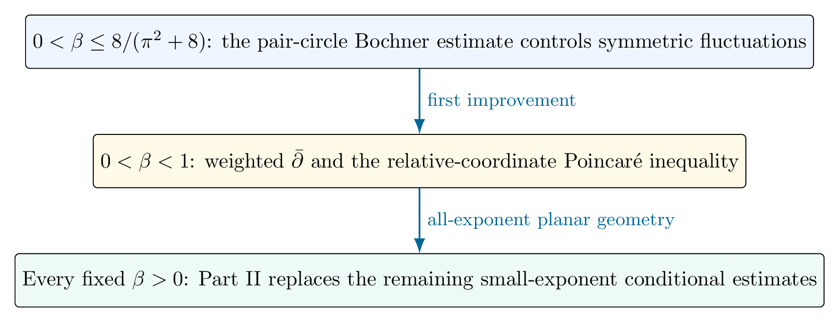
The weighted Dolbeault estimate will play an important role in the all-temperature proof. What Part II replaces are the one-site logarithmic Sobolev inequality and the relative-coordinate Poincaré inequality when the total exponent is no longer small.
6.2 Where the plane enters
Exponentiating a logarithmic interaction always produces products of distance powers, so that feature alone is not uniquely two-dimensional. The planar structure enters in the way we exploit those products.
First, for a moving pair in the plane, the relative coordinate is one complex scalar. At fixed radius, its angular variable lies on a circle, and the Bochner estimate uses a weighted Wirtinger inequality for a \(\pi\)-antiperiodic function on that circle. Higher-dimensional \(A_2\) theory exists, but the scalar factorization and the exact circle argument do not survive unchanged when the angular variable lies on a higher-dimensional sphere.
Second, the collision factor is the modulus of the holomorphic Vandermonde polynomial. Away from collisions, \(\log|\Delta_N|\) is pluriharmonic and therefore contributes nothing to the Levi curvature in the weighted dbar estimate. In higher real dimension, even after choosing a complex structure, the logarithm of the Euclidean norm is not pluriharmonic away from the origin and the pair interaction is not the modulus of a scalar holomorphic linear factor. The holomorphic rigidity argument has no direct analogue.
Finally, the all-temperature conditional theorem described in Part II uses quasiconformal and strong-\(A_\infty\) geometry, together with weak-\(L^2\) control of the logarithmic field and the Ladyzhenskaya inequality. These are again specifically two-dimensional. For nonlogarithmic Riesz interactions, there is an earlier obstruction: exponentiating the interaction no longer produces algebraic distance factors at all.
Remark. Remark 8 (Perturbative extensions beyond the plane). The preceding limitations concern the particular planar approach developed here, not the perturbative regime itself. Related perturbative arguments also give \(N\)-uniform logarithmic Sobolev inequalities at sufficiently small \(\beta\) for higher-dimensional Coulomb gases and for a range of non-Coulomb Riesz interactions at the same diffusive temperature scale. We do not pursue these extensions here, since our ultimate objective is an \(N\)-uniform inequality for every fixed \(\beta>0\). At present, we have reached this all-temperature regime only for the planar Coulomb gas, although preliminary calculations for the three-dimensional Coulomb gas suggest that a similar all-temperature result holds there as well.
6.3 Why the perturbative argument stops
The improvement to \(\beta<1\) removes the numerical Bochner threshold, but the perturbative method still reaches structural limits.
6.3.0.1 Weighted thresholds.
For \(|x|^q\) in the plane, the reciprocal weight ceases to be locally integrable at \(q=2\). On the radial one-dimensional slices used for the one-site LSI, the corresponding threshold is \(q=1\). Once the conditional total exponent crosses these values, the \(A_2\) proof is no longer available. This is a failure of the criterion, not evidence that the conditional Poincaré or logarithmic Sobolev inequality itself fails.
6.3.0.2 Curvature thresholds.
The first permutation-invariant argument required
\[ 1-\frac\beta2\frac{\pi^2}{4(1-\beta)}\ge0. \tag{6.13} \]
The paired circle estimate remains available for \(0<\beta<1\), but its absolute-value Bochner absorption coefficient is negative when \(\beta_{\mathrm B}<\beta<1\). Thus, the obstruction beyond \(\beta_{\mathrm B}\) is failure of this absorption, not failure of reciprocal integrability. Independently, the label-dependent part of the first proof uses the two-particle conditional logarithmic Sobolev inequality, which is available here only for \(\beta<1/2\). Pointwise Bakry–Émery curvature cannot repair this because \(D^2(-\log|z|)\) has one positive and one negative eigenvalue of inverse-square size. One might instead hope that, after integrating the Bochner identity against the Gibbs law, the positive Hessian term compensates the negative Coulomb-curvature term separately for each particle pair. This fails for arbitrary labeled observables: for the two-particle relative test \(v(r,\theta)=r e^{-cr^2}\cos\theta\), at \(\beta=1\) and \(c=1/100\), the resulting two-particle form has the sign of
\[ -\frac{36643}{8652800}<0. \tag{6.14} \]
Thus, the desired pair-by-pair compensation is false for arbitrary labeled observables. Exchanging the two particle labels sends the relative coordinate \(u\) to \(-u\) and changes the sign of this test, so the example does not address permutation-invariant observables, which are unchanged by that exchange. For \(N\ge3\), contributions from different particle pairs may also compensate after summation, a possibility that the two-particle calculation cannot test.
6.3.0.3 Finite-block reconstruction.
Suppose one proves integrated Bochner estimates after conditioning on all blocks \(I\subset\{1,\ldots,N\}\) of a fixed size \(k\) and then averages the resulting estimates. A coordinate belongs to a fraction \(k/N\) of the blocks, whereas a pair belongs to a fraction \(k(k-1)/(N(N-1))\). After normalizing the one-coordinate term to have coefficient one, the pair-Hessian term is multiplied by
\[ \frac{k-1}{N-1}. \tag{6.15} \]
Uniformly good estimates on fixed-size blocks cannot, by positive averaging alone, recover the full pair-interaction Hessian term in the \(N\)-particle Bochner identity: after normalizing the one-coordinate term, every pair contribution is reduced by the factor \((k-1)/(N-1)\), which vanishes for fixed \(k\).
These obstructions identify the two estimates that must be replaced: the one-site logarithmic Sobolev inequality and the relative-coordinate Poincaré inequality when the total exponent is no longer small. Part II proves a planar weighted theorem which, when applied to the one-site and relative-coordinate conditional measures, yields both replacement estimates.
7 Consequences, neighboring models, and the problem behind Part II
The most distinctive consequence of Theorem 1.1 is the space on which the inequality holds. It acts on every labeled observable, not only on functions of the empirical measure. For example, exchangeability gives \(\mathbb E_{\mathbb P_{N,\beta}}[\varphi(z_1)-\varphi(z_2)]=0\), and the Poincaré consequence of the theorem yields
\[ \mathbb E_{\mathbb P_{N,\beta}} \left[\bigl(\varphi(z_1)-\varphi(z_2)\bigr)^2\right] \le\frac1{\rho_\beta} \mathbb E_{\mathbb P_{N,\beta}} \left[|\nabla\varphi(z_1)|^2+|\nabla\varphi(z_2)|^2\right]. \tag{7.1} \]
For nonconstant \(\varphi\), the tagged observable \(\varphi(z_1)-\varphi(z_2)\) is not determined by the empirical measure. Consequently, an inequality restricted to test functions of the empirical measure does not apply to this observable directly. Dynamically, the same distinction means that entropy decay applies to finite-entropy initial laws that are not exchangeable, and therefore controls perturbations carrying information in the particle labels.
The usual consequences now remain uniform as the dimension \(2N\) grows. The physical generator is
\[ L_{N,\beta}^{\mathrm{phys}} =\frac1\beta\Delta-\nabla \mathcal H_N\cdot\nabla =\frac1\beta\mathcal L, \tag{7.2} \]
and the LSI gives
\[ \mathcal H(\nu_t\mid \mathbb{P}_{N,\beta}) \le e^{-2\rho_\beta t/\beta} \mathcal H(\nu_0\mid \mathbb{P}_{N,\beta}). \tag{7.3} \]
Thus, the entropic relaxation time does not diverge solely because \(N\) increases. This does not imply an \(N\)-independent total-variation mixing time from arbitrary initial data, since the initial entropy may grow like \(N\) or be infinite.
Similarly, for a Lipschitz function \(\varphi:\mathbb C\to\mathbb R\) and
\[ F_N(Z):=\frac1N\sum_{i=1}^N\varphi(z_i), \tag{7.4} \]
one has
\[ |\nabla F_N|^2 \le\frac{\mathop{\mathrm{Lip}}(\varphi)^2}{N}. \tag{7.5} \]
Herbst’s argument therefore gives the natural order-\(N\) concentration exponent
\[ \mathbb{P}_{N,\beta}\bigl(|F_N-\mathbb E_{\mathbb{P}_{N,\beta}}[F_N]|\ge r\bigr) \le2\exp\!\left(-\frac{\rho_\beta N r^2} {2\mathop{\mathrm{Lip}}(\varphi)^2}\right). \tag{7.6} \]
A fixed-\(N\) inequality with \(\rho_{N,\beta}\to0\) would not retain either (7.3) or (7.6) at these scales.
Uniform finite-particle LSIs are also the natural microscopic coercivity estimate in the modulated logarithmic Sobolev approach to generation of chaos [RS25]. The equilibrium theorem proved here is not by itself a complete dynamical propagation-of-chaos result: one must still compare the particle law with the evolving mean-field reference and control the corresponding modulated entropy production. It does, however, supply the full labeled equilibrium endpoint rather than only a symmetric or empirical-measure inequality.
7.1 Why quadratic confinement matters
Our first proof uses four special features of isotropic quadratic confinement. Some individual features persist under broader assumptions—for example, uniform convexity supplies curvature lower bounds—but uniform convexity alone does not provide exact center-of-mass factorization, the Gaussian conditional form, or common-phase symmetry.
Exact center-of-mass factorization. Translation invariance of the interaction and orthogonality of the quadratic form separate a Gaussian center-of-mass factor without loss.
Stable conditional form. After freezing particles or a pair center, the remaining law is a centered Gaussian multiplied by products of distance powers. A general confinement introduces environment-dependent affine and nonlinear terms.
Constant real and complex curvature. The integrated Bochner identity contains the exact positive term \(\beta\int|\nabla f|^2\), while the weighted dbar estimate has the exact Levi lower bound \(\beta/2\).
Common-phase symmetry. The transformation \(Z\mapsto e^{i\theta}Z\) preserves both confinement and interaction and is used in the holomorphic rigidity argument.
7.2 A perturbative periodic companion
A parallel perturbative theorem holds on the square torus, although the Poincaré proof changes. Recycling notation, let \(\mathbb P_{N,\beta}\) be the Gibbs measure on \((\mathbb T^2)^N\) with \(\mathsf g\) given by the mean-zero Green function
\[ -\Delta \mathsf g=2\pi(\delta_0-1), \qquad \int_{\mathbb T^2}\mathsf g=0, \tag{7.7} \]
and
\[ \,\mathrm d\mathbb P_{N,\beta}(X_N) \propto \exp\!\left[-\frac\beta{2N}\sum_{i\ne j}\mathsf g(x_i-x_j)\right] \,\mathrm dx_1\cdots\,\mathrm dx_N. \tag{7.8} \]
Let \(\beta_D>0\) be the unique positive solution of
\[ \beta_D\,\frac{\sqrt2}{2} \left(\int_{\mathbb T^2}|\nabla\mathsf g(x)|\,\mathrm dx\right) \exp\!\left(-\beta_D\inf_{\mathbb T^2}\mathsf g\right)=1. \tag{7.9} \]
Proposition 7.1 (Perturbative periodic companion). *For
\[ 0<\beta<\min\{2,\beta_D\}, \tag{7.10} \]
the Gibbs measure \(\mathbb P_{N,\beta}\) satisfies a logarithmic Sobolev inequality with a constant bounded below independently of \(N\).*
To obtain the one-site conditional inequalities on the torus, one first works in Euclidean coordinate charts. The local analytic input is the Fabes–Kenig–Serapioni weighted Poincaré inequality: if \(B\subset\mathbb R^2\) is a ball of radius \(r\), \(w\in A_2\), and
\[ h_{B,w}:=\frac{\int_Bh\,w\,\mathrm dx}{\int_Bw\,\mathrm dx}, \tag{7.11} \]
then
\[ \int_B|h-h_{B,w}|^2w\,\mathrm dx \le C\bigl([w]_{A_2}\bigr)r^2 \int_B|\nabla h|^2w\,\mathrm dx. \tag{7.12} \]
One also uses the corresponding weighted Sobolev estimate; see [FKS82, Section 1]. A finite coordinate cover transfers these inequalities to the torus once the conditional weights have a uniform \(A_2\) bound.
The conditional LSI and the partition estimate are then used as in the confined case. What changes is the spectral-gap argument: the torus has no positive confinement Hessian and no Gaussian center-of-mass factor, so a Dobrushin–Wu influence contraction [Wu06] replaces the harmonic Bochner estimate. This comparison separates the parts of the perturbative argument that survive on compact geometry from those tied to quadratic confinement.
7.3 The problem behind Part II
The perturbative analysis reduces the remaining difficulty to a one-particle statement. Consider
\[ \,\mathrm d\nu(z) =\frac1Z e^{-\gamma|z|^2/2} \prod_{j=1}^m|z-y_j|^{a_j}\,\mathrm dz, \qquad a_j\ge0, \qquad \sum_{j=1}^ma_j\le Q<\infty. \tag{7.13} \]
The preceding measure models both the law of one particle conditioned on all the others and the law of a pair’s relative coordinate conditioned on the pair center and all remaining particles. In either application, the number of distance factors grows with the particle number and their centers may coalesce; only the total exponent remains uniformly bounded. The \(A_2\) proof controls (7.13) only while reciprocal-weight estimates remain available.
The theorem proved in Part II is that, for every \(\gamma>0\) and every finite \(Q\), the measures in (7.13) satisfy Poincaré and logarithmic Sobolev inequalities with constants depending only on \((\gamma,Q)\), uniformly in \(m\), the locations and multiplicities of the points \(y_j\), and their clustering. Its local part uses quasiconformal Jacobians and strong-\(A_\infty\) weights [BL03, Bjö01, DS90]; its global part combines Gaussian confinement with weak-\(L^2\) control of the logarithmic field and the Ladyzhenskaya inequality (see, e.g., [FMRT01, Chapter I, Section 4, equation (4.8)]).
Once this theorem is inserted into the one-site and relative-coordinate conditionals, the weighted dbar argument continues to control permutation-invariant fluctuations, while the transposition estimate, conditional entropy argument, partition bound, and Rothaus tightening remain unchanged. The proof of that weighted planar theorem and its insertion into the many-particle argument above will be the subject of Part II.
7.4 References
[ABC+00] C. Ané, S. Blachère, D. Chafaï, P. Fougères, I. Gentil, F. Malrieu, C. Roberto, and G. Scheffer, Sur les inégalités de Sobolev logarithmiques, Panoramas et Synthèses 10, Société Mathématique de France, 2000.
[AV65] A. Andreotti and E. Vesentini, Carleman estimates for the Laplace–Beltrami equation on complex manifolds, Publ. Math. Inst. Hautes Études Sci. 25 (1965), 81–130. doi:10.1007/BF02684398.
[BBD25] R. Bauerschmidt, T. Bodineau, and B. Dagallier, A criterion on the free energy for log-Sobolev inequalities in mean-field particle systems, arXiv:2503.24372, 2025.
[BCF18] F. Bolley, D. Chafaï, and J. Fontbona, Dynamics of a planar Coulomb gas, Ann. Appl. Probab. 28 (2018), no. 5, 3152–3183. doi:10.1214/18-AAP1386.
[BGL14] D. Bakry, I. Gentil, and M. Ledoux, Analysis and Geometry of Markov Diffusion Operators, Grundlehren der mathematischen Wissenschaften 348, Springer, 2014. doi:10.1007/978-3-319-00227-9.
[Bjö01] J. Björn, Poincaré inequalities for powers and products of admissible weights, Ann. Acad. Sci. Fenn. Math. 26 (2001), no. 1, 175–188.
[BL03] M. Bonk and U. Lang, Bi-Lipschitz parameterization of surfaces, Math. Ann. 327 (2003), 135–169. doi:10.1007/s00208-003-0443-8.
[CG14] P. Cattiaux and A. Guillin, Functional inequalities via Lyapunov conditions, in Optimal Transportation: Theory and Applications, London Math. Soc. Lecture Note Ser. 413, Cambridge Univ. Press, 2014, 274–287.
[CG17] P. Cattiaux and A. Guillin, Hitting times, functional inequalities, Lyapunov conditions and uniform ergodicity, J. Funct. Anal. 272 (2017), no. 6, 2361–2391. doi:10.1016/j.jfa.2016.10.003.
[CGWW09] P. Cattiaux, A. Guillin, F.-Y. Wang, and L. Wu, Lyapunov conditions for super Poincaré inequalities, J. Funct. Anal. 256 (2009), no. 6, 1821–1841. doi:10.1016/j.jfa.2009.01.003.
[CL20] D. Chafaï and J. Lehec, On Poincaré and logarithmic Sobolev inequalities for a class of singular Gibbs measures, in Geometric Aspects of Functional Analysis, Lecture Notes in Mathematics 2256, Springer, 2020, 219–246. doi:10.1007/978-3-030-36020-7_10.
[CNZ24] S. Chewi, A. Nitanda, and M. S. Zhang, Uniform-in-\(N\) log-Sobolev inequality for the mean-field Langevin dynamics with convex energy, SIAM J. Math. Anal. 58 (2026), no. 4, 3652–3668. doi:10.1137/24M1696068.
[Dem12] J.-P. Demailly, Complex Analytic and Differential Geometry, open-content book, Université de Grenoble I, Institut Fourier, version of June 21, 2012. Author’s online PDF.
[DG25] M. G. Delgadino and R. S. Gvalani, Sharp mean-field estimates for the repulsive log gas in any dimension, arXiv:2506.22083, 2025.
[DGR] M. G. Delgadino, R. S. Gvalani, and M. Rosenzweig, Sharp mean-field estimates for diffusive log/Riesz gases in the Hilbert–Schmidt regime, in preparation.
[DJ26] M. Duerinckx and P.-E. Jabin, Singular mean-field limits for fluctuations around equilibrium, arXiv:2605.28979, 2026.
[DS81] P. Diaconis and M. Shahshahani, Generating a random permutation with random transpositions, Z. Wahrscheinlichkeitstheorie verw. Gebiete 57 (1981), 159–179. doi:10.1007/BF00535487.
[DS90] G. David and S. Semmes, Strong \(A_\infty\) weights, Sobolev inequalities and quasiconformal mappings, in Analysis and Partial Differential Equations, Lecture Notes in Pure and Appl. Math. 122, Dekker, 1990, 101–111.
[FKS82] E. B. Fabes, C. E. Kenig, and R. P. Serapioni, The local regularity of solutions of degenerate elliptic equations, Comm. Partial Differential Equations 7 (1982), no. 1, 77–116. doi:10.1080/03605308208820218.
[FMRT01] C. Foias, O. Manley, R. Rosa, and R. Temam, Navier–Stokes Equations and Turbulence, Encyclopedia of Mathematics and its Applications 83, Cambridge University Press, Cambridge, 2001. doi:10.1017/CBO9780511546754.
[FOT11] M. Fukushima, Y. Oshima, and M. Takeda, Dirichlet Forms and Symmetric Markov Processes, second revised and extended edition, De Gruyter Studies in Mathematics 19, Walter de Gruyter, Berlin, 2011. doi:10.1515/9783110218091.
[GLWZ22] A. Guillin, W. Liu, L. Wu, and C. Zhang, Uniform Poincaré and logarithmic Sobolev inequalities for mean field particle systems, Ann. Appl. Probab. 32 (2022), no. 3, 1590–1614. doi:10.1214/21-AAP1707.
[GOVW09] N. Grunewald, F. Otto, C. Villani, and M. G. Westdickenberg, A two-scale approach to logarithmic Sobolev inequalities and the hydrodynamic limit, Ann. Inst. H. Poincaré Probab. Statist. 45 (2009), no. 2, 302–351. doi:10.1214/07-AIHP200.
[GR20] F. Grotto and M. Romito, A central limit theorem for Gibbsian invariant measures of 2D Euler equations, Comm. Math. Phys. 376 (2020), no. 3, 2197–2228. doi:10.1007/s00220-020-03724-1.
[Gra14] L. Grafakos, Classical Fourier Analysis, 3rd ed., Graduate Texts in Mathematics 249, Springer, New York, 2014. doi:10.1007/978-1-4939-1194-3.
[Gro75] L. Gross, Logarithmic Sobolev inequalities, Amer. J. Math. 97 (1975), no. 4, 1061–1083. doi:10.2307/2373688.
[GZ03] A. Guionnet and B. Zegarlinski, Lectures on logarithmic Sobolev inequalities, in Séminaire de Probabilités XXXVI, Lecture Notes in Mathematics 1801, Springer, 2003, 1–134.
[Han78] T. S. Han, Nonnegative entropy measures of multivariate symmetric correlations, Information and Control 36 (1978), no. 2, 133–156. doi:10.1016/S0019-9958(78)90275-9.
[Hör65] L. Hörmander, \(L^2\) estimates and existence theorems for the \(\bar\partial\) operator, Acta Math. 113 (1965), 89–152. doi:10.1007/BF02391775.
[HS87] R. Holley and D. W. Stroock, Logarithmic Sobolev inequalities and stochastic Ising models, J. Statist. Phys. 46 (1987), 1159–1194. doi:10.1007/BF01011161.
[Led01] M. Ledoux, The Concentration of Measure Phenomenon, Mathematical Surveys and Monographs 89, American Mathematical Society, 2001.
[LM20] Y. Lu and J. C. Mattingly, Geometric ergodicity of Langevin dynamics with Coulomb interactions, Nonlinearity 33 (2020), no. 2, 675–699. doi:10.1088/1361-6544/ab514a.
[Mon24] P. Monmarché, Uniform log-Sobolev inequalities for mean field particles beyond flat-convexity, arXiv:2409.17901, 2024.
[MS14] G. Menz and A. Schlichting, Poincaré and logarithmic Sobolev inequalities by decomposition of the energy landscape, Ann. Probab. 42 (2014), no. 5, 1809–1884. doi:10.1214/14-AOP908.
[Muc72] B. Muckenhoupt, Weighted norm inequalities for the Hardy maximal function, Trans. Amer. Math. Soc. 165 (1972), 207–226. doi:10.2307/1995882.
[OR07] F. Otto and M. G. Reznikoff, A new criterion for the logarithmic Sobolev inequality and two applications, J. Funct. Anal. 243 (2007), no. 1, 121–157. doi:10.1016/j.jfa.2006.10.002.
[Rot85] O. S. Rothaus, Analytic inequalities, isoperimetric inequalities and logarithmic Sobolev inequalities, J. Funct. Anal. 64 (1985), no. 2, 296–313. doi:10.1016/0022-1236(85)90079-5.
[RS25] M. Rosenzweig and S. Serfaty, Modulated logarithmic Sobolev inequalities and generation of chaos, Ann. Fac. Sci. Toulouse Math. 34 (2025), no. 1, 107–134. doi:10.5802/afst.1807.
[Ser24] S. Serfaty, Lectures on Coulomb and Riesz Gases, American Mathematical Society Colloquium Publications, vol. 70, American Mathematical Society, Providence, RI, 2026. doi:10.1090/coll/070.
[Wan24] S. Wang, Uniform log-Sobolev inequalities for mean field particles with flat-convex energy, arXiv:2408.03283, 2024.
[Wu06] L. Wu, Poincaré and transportation inequalities for Gibbs measures under the Dobrushin uniqueness condition, Ann. Probab. 34 (2006), no. 5, 1960–1989. doi:10.1214/009117906000000368.
Citation
@online{rosenzweig2026,
  author = {Rosenzweig, Matthew},
  title = {Uniform Logarithmic {Sobolev} Inequalities for the {2D}
    {Coulomb} Gas at the Diffusive Temperature Scale, {Part} {I}},
  date = {2026-08-11},
  url = {https://matthewrosenzweigwork-max.github.io/posts/uniform-logarithmic-sobolev-2d-coulomb-gas-part-i/},
  langid = {en}
}